VLOOKUP Formulas in Microsoft Excel
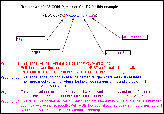
The following graphic provides a breakdown for a VLOOKUP formula, and describes each argument. It may be helpful to review it before you continue reading the rest of the article. The V in VLOOKUP means "vertical". HLOOKUP works similarly, but finds data going across columns, instead of down rows.
VLOOKUP has many purposes. You can quickly create a pricelist that is thousands of rows long on Sheet2. On Sheet1, you can designate a cell into which to type a part number, and then have a VLOOKUP that finds the price on Sheet2. No scrolling, no need to use the Find feature to find the price for the part.
The following graphic demonstrates how to look up the salary of only several employees. Note that the VLOOKUP formula in cell D2 is shown in the formula bar.

So, what's MyLookup? That's our data range or database" where the Salary table lies, which is demonstrated in the following graphic.

In the above, columns A through G were selected, and a named range was created by hitting Insert - --
People often get errors when performing VLOOKUPs. Here's a few common errors and the reasons for them.
#N/A.
When you get this error, it means that the formula is not finding the value that you're looking for in the list in which you're looking. In our example, that means that the value in A2 was not found in the first column of the Employee Data sheet. Unfortunately, you may also get this error if you are looking for a number, and your numbers are formatted as text. You can test this theory: Create a new workbook. Format column A as text. Format column B as a custom format with 000000 as the custom format. Now, type '000123 in cell A1 (don't miss the apostrophe before the first zero there) and type 123 in B1. Both values *look* the same. However, you have 7 characters in cell A1 and only 3 characters in B1. Trying to do a VLOOKUP under these circumstances will not work. This happens often when you get data from an *external data source*, such as a mainframe database. Basically, VLOOKUP works best when the values you're looking for and the values you're looking in both have the same format. To repair this, you must do the following procedure to one or both of the data ranges of numbers. We call it *The Copy Blank Fix* for lack of a better title. The Copy Blank fix. Copy any blank cell. Select the range of numbers or dates that may be causing the error. Hit Edit Paste special, and choose Add. Hit OK. Your range will likely lose its formatting and need to be formatted again. However, this FORCES Excel to see the data as numbers or date values instead of as text.
Wrong Value Returned
This is usually caused by not including the FALSE (or fourth) argument in the VLOOKUP formula. If your data lookup column is not sorted, your formula may find the closest value it first comes across, unless you use the FALSE statement. One of the few times a FALSE statement should NOT be used is if you have a range of values that relate to another range of values. Suppose we have insurance premiums that are $1.00 per month up to age 16, $2.00 per month up to age 21, and so on. You might have the first column be the ages, i.e., 16, 21, 25, etc. Now suppose the value you are looking up is 20. It should then return the nearest match without going over, which would be the same amount as for a lookup value of 16, or $1.00 in this case. Change the value you are looking up to 22 and it will find the 21-year-old value.
Bad Range
This is a common issue. Our VLOOKUP sample shows how to create the formula using named ranges. However, probably more commonly used is the referenced range. In this case, it would be A1:G7 of the Employee Data sheet. So instead of =VLOOKUP(A2,MyLookup,2,FALSE) our formula would read =VLOOKUP(A2,Employee Data!$A$1:$G$7,2,FALSE). Many people forget to put the dollar signs in to keep the range ABSOLUTE. In other words, when they copy the formula down one cell, instead of getting: =VLOOKUP(A3,Employee Data!A1:G7,2,FALSE) , they get =VLOOKUP(A2,Employee Data!A2:G8,2,FALSE) because they did not use the dollar signs. This is why it is so much easier to use a named range. And also to use entire columns when naming the range.
