An Extreme Tutorial in Microsoft Excel
This tutorial covers the features and tasks most commonly asked about in the
newsgroups and in technical support forums all over the internet. Hopefully, by
taking this tutorial, you'll learn a lot about Excel very quickly.
We assume that you know the difference between a cell, a worksheet and a workbook. We assume you know how to type and use a mouse.
The steps must be taken in the order provided to get the exact results displayed. This tutorial is presented in Excel 2003.
Set Your Menu
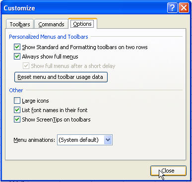
To be sure you can follow the instructions exactly, you should first set your menus as follows. Go to Tools Customize from the menu and click on the Options tab. Check the top two checkboxes.
Download the Files
To properly perform the exercises provided in this tutorial, you must first download the files for it by clicking here. The files are stored in a Zip file. Download the zip file to your computer. Right-click the zip file and hit Extract. Extract the entire folder to a familiar location on your hard drive; usually My Documents.
Open SampleData.xls
From Excel's menu, hit File Open and choose the file called SampleData.xls. The data is not real in any way.
As you work through this tutorial, you may want to occasionally save your file. You can do it by hitting the Save diskette on the Standard toolbar, or by hitting Ctrl+S.
Sort the Data
Click on cell D2. From the Standard toolbar, choose the Sort Ascending button.
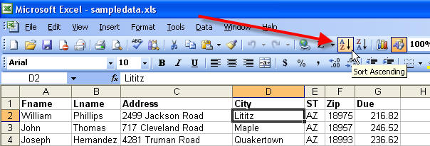
The cities become sorted alphabetically in ascending order.
Click on cell G2, and hit the Sort Descending button.
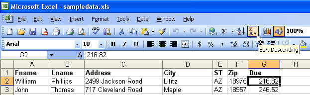
See the result. I do not show all records.
If the sorting function does not work for you, perhaps Excel doesn't realize you have headings in row 1. Let it know by going to Data Sort and choosing the Header Row option.
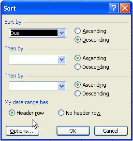
Now you realize you can sort by several columns at once. So go ahead and sort by Last Name, then by First Name, then by City, all ascending.
See the result, which becomes much more apparent if you change some of the last names to be the same. I do not show all records.
If you need to sort by more than 3 columns, see this article to learn how.
Save the file.
AutoFilter the Data
You need to find just one person's name quickly? Hit Data Filter AutoFilter. From the Last Name column, hit the dropdown, and hit the letter L on your keyboard. Choose Lee with your mouse.
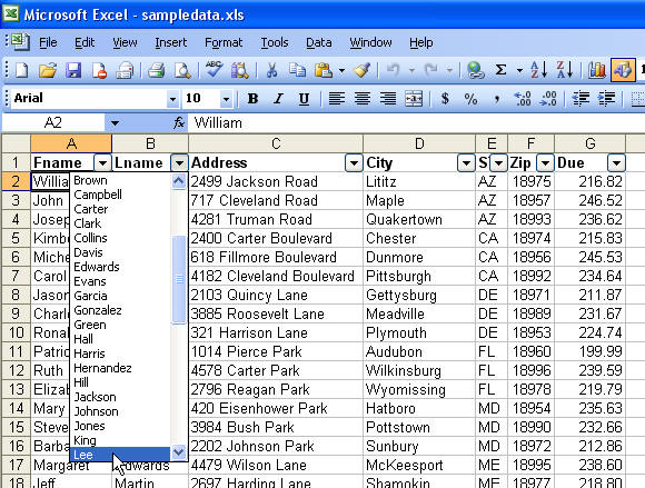
See the result. We only see one record because only one person has that last name. We would see all persons listed with that last name.
Now hit the dropdown arrow on Last Name again, and choose All to see all records again. Then hit the dropdown on the Due column. Choose Custom. Change the first drop-down to Is greater than, and type 225.00 into the right-hand box.
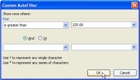
See the result. I do not show all records.
Hit the drop-down and choose All to show all records again. Choose the State drop-down (Column E), and choose AZ, then choose the Due drop-down and again do a custom filter for values greater than 225.00. Here is the result. This time, I show all records.
Turn off AutoFilter by going to Data Filter AutoFilter. All filters and their arrows are removed.
Save the file.
Concatenate the Data
I don't want to get into too many formulas, but this is very helpful, even to the noobie. Click on cell H1 and type "FullName". In cell H2, type the following formula and hit Enter.
=A2&" "&B2
Note that you do not have to type the formula using capital letters. Excel will convert them for you if your cell references are valid.
Now click on cell H2 and double-click the bottom, right-hand corner of the cell to copy this formula down to all cells that contain data in the adjacent (Due) column. The result is we now have everyone's name in one column. However, if you delete column A and B now, you'll be in trouble.
Save the file.
Paste Special Values
While the cells are still selected (highlighted, but we don't call it that!), hit Ctrl+C to copy it. Then, without deselecting the cells, go to the Edit menu and choose Paste Special Values. Now, if you wanted to, you could safely delete columns A and B.
Save the file.
Auto-Resize Columns
Column H isn't wide enough to hold the names. You can resize the columns using the methods in this article, or-since we only need to fix the width of one column-you can just double-click the line between H and I columns. You know your cursor is in position when it gets the two-way arrow.
Save the file.
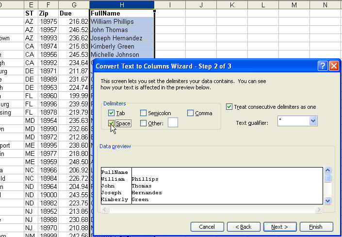
Data Text to Columns
We've learned how to put two names together. However, it seems that even more than doing that, people need to split names up. Perhaps so they can do a mail merge to Dear John instead of to Dear John Smith. Here's how we separate them, which works in many, but not all cases. If nothing else, it can make a really long manual chore take a whole lot less time.
Place your cursor on the H and click to select the entire column H. Go to the menu and choose Data Text to Columns.
Choose Delimited and hit Next. Then tick the Space checkbox. This tells Excel that spaces are what separates the data. Note the data preview. Hit Finish.
Warning: If you have data in the column(s) to the right when you use this feature, you could wipe it out.
See the result.
Save the file.
Delete Columns
We won't use columns H and I anymore, so let's delete them. Click on the letter H and drag to the right to select I, too. From the menu, choose Edit Delete.
Choose rows 5, 6 and 7, and from the menu, choose Edit Delete.
Save the file.
Quick Functions
Click in cell G2, and hit Shift+Ctrl plus the down arrow key. This should select cells G2 through G48. Alternatively, you can hit F5 and type G2:G48 into the box and hit Enter.
On the right-hand side of the status bar, note what it says.
Now, right-click where it says Sum= and choose Count.

Right-click again and choose some of the other options. When you're done, hit Ctrl+Home to get to the top of your worksheet.
Save the file and close it.
An Exercise for the Boss
Open the file called PriceList.xls.
This particular exercise contains the VLOOKUP formula, which is so widely used, and so difficult for many to understand. It is the hardest Excel task I ever learned. But once you learn it, you'll never forget again how to use it-as long as you keep using it! Please follow the steps carefully.
The boss provides you with the current price list and asks you to make it easier to find a price. He says he doesn't care how you do it, just get it done. He is sure that this "MicroStock Office" must have an easier way to make a price list that's easier to find prices with. And he's right.
We want to find a part number, then look to the right of it to find its price. We're going to use the VLOOKUP formula. For an overview of VLOOKUP, see this article.
A couple of rules about VLOOKUP:
-
It only looks at the data from left to right.
-
It only returns one value.
Our part number is in the far right column. This is not good. It doesn't follow our first rule. So we must move the part number. We'll make it easy and put our part number in the far left column.
Move a Column
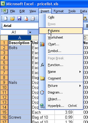
Click on the letter A to select column A, and hit Insert Column.
Now click on column E to select the column, and then place your cursor just between the E and the first cell in column E, as shown:
Drag E over to replace the blank A column. See the result.
Fill Empty Cells
No decent Excel data file really has grouped values and looks like a report. Every good Excel database has all the values filled in where appropriate. So we need to copy the values in column B into any blank cells of column B. I explain this in detail in this article. But we'll go through the steps here.
-
Hit F5 or Ctrl+G to bring up the GoTo box.
-
Type in B2:B48 and hit Enter.
-
Hit Edit GoTo Special Blanks.
-
Type =B2 and hit Ctrl+Enter.
-
Keep the cells selected and hit Ctrl+C to copy, then Edit Paste special, Values, OK.
-
Hit Ctrl+Home.
-
Sort ascending by column A.
-
Save the file.
Insert and Name a Worksheet
Double-click Sheet1's tab and rename it to Pricelist. Left-click on Sheet2's tab and drag it to the left of Sheet1's tab and rename Sheet2 to Lookup.
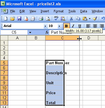
On your new Lookup worksheet, make it look just like this one.
Bold the cells the labels are in and widen column C.
Format Painter
Format the cells as they are formatted on the PriceList worksheet. You can do this by using the Format Painter. Click here for more information on the Format Painter.
-
Go to the PriceList worksheet by clicking on its sheet tab. Click on any price, then click on the Format Painter.
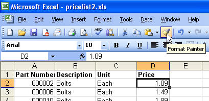
-
Go back to the Lookup worksheet by clicking on its tab and click on cell D11 to apply the formatting to it.
-
Format D13 the same as D11.
-
Format D5 the same as the PriceList worksheet, cell A2.
Using the Borders toolbar button, select D5, and put a Thick Box Border on it.
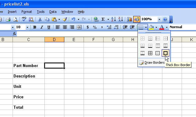
Click on cell D7 and hit the F4 key. Click on Cell D9 and hit the F4 key, and so on until each item has a box around the cell. Widen Column D.
Save the file.
Do the VLOOKUP
We're going to do more than the boss asked for.
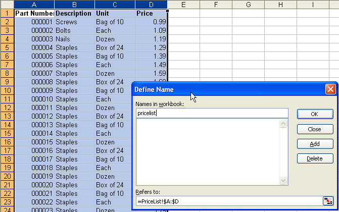
-
In the PriceList worksheet, select columns A through D and hit Insert Name Define and type pricelist (all one word, no spaces-see more on naming ranges here).
-
Go back to the Lookup worksheet and type a 1 in cell D5.
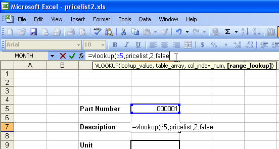
-
Following the instructions and syntax of our VLOOKUP article, we'll type the following formula into cell D7.
=VLOOKUP(D5,pricelist,2,false)
-
Copy D7, and paste it into cells D9 and D11. (Alternatively, if you copy the formula from the formula bar, and paste into D9 and D11, you'll have a little bit less editing to do.)
-
Edit the formula D9 to look in D5 (instead of D7) and to look in column 3 (instead of column 2).
-
Edit the formula in D11 to look in D5 (instead of D9) and to look in column 4 (instead of column 2).
-
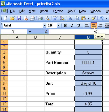
Add a Quantity label and box above the Part Number (yep, I forgot it). Type a quantity into cell D3.
-
Select Column D and hit the Center button on the Formatting toolbar.
-
In cell D13, type the following formula.
=D3*D11
Pretty cool, right? But what happens if we delete the part number? Yuk!
Save the file.
Error Handling in Formulas
In cell D7, change the formula to read:
=IF(ISBLANK(D5),"",VLOOKUP(D5,pricelist,2,FALSE))
Change D9 and D11 in the same way. The "" part means, basically, show nothing. If you want a zero to show, put a zero instead of the quotes.
Think you can change D13, too? Go ahead.
Another formula that will work better in other circumstances:
=IF(ISNA(VLOOKUP(D5,pricelist,2,FALSE)),"",VLOOKUP(D5,pricelist,2,FALSE))
You can use that formula if you have a calculation in D5, and it's not really blank. It doesn't suit this particular situation, but I wanted to include the ISNA function here. Also try ISERROR.
Drop-Down Using Data Validation
I cover this in detail here, but wanted to put it into this tutorial anyway.
-
Go to the PriceList worksheet and click on cell A2, and hit Shift+Ctrl plus the down arrow key to select all the part numbers.
-
From the menu, hit Insert Name Define and type partnos and hit Enter.
-
Go back to the Lookup worksheet and select cell D5. From the menu, choose Data Validation.
-
From the dropdown, choose List, and type into the box: =partnos
-
Hit OK.
Play with the dropdown box choosing part numbers.
Watch it fill in.
Enter a quantity and watch it fill in.
Click on Cell A1 and hit Format Row Height and type 24 into the box, and hit OK.
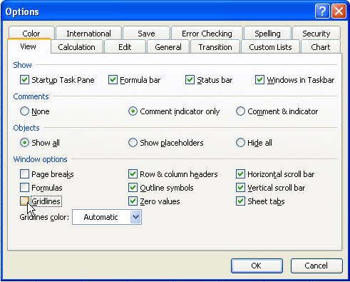
Change the font to 18 pt bold and blue. Type Price Lookup into the cell. Go to Tools Options, View tab, and uncheck gridlines.
See the result.
Want to clear the quantity and part number? You can record that as a macro, and then assign it to a button.